This TensorFlow tutorial explains What is TensorFlow, its APIs, and its Application along with the step-by-step installation process for your easy understanding:
What is TensorFlow?
TensorFlow was designed by the analysts and engineers of the Google Brain Team for inner Google purposes, such as for production and research. It is an open-source and free library used for machine learning and artificial intelligence.
TensorFlow can be employed over wide-ranging tasks but its primary focus is on training and speculation of deep neural networks. It is used to conduct research for machine learning and deep neural networks, but it can be implemented in various other domains as well.
TensorFlow is used in numerous programming languages, which incorporate Python, JavaScript, C++, and Java.
Table of Contents:
Google TensorFlow Tutorial: Hands-On Review

TensorFlow is a second-generation system, by Google Brain. It can function on various CPUs as well as GPUs. It is accessible across computing platforms such as Android and iOS. Its versatile framework enables easy distribution of computation across diverse platforms, from desktops to collections of servers to mobile and border devices.
The TensorFlow platform assists in implementing the best applications for data automation, model tracking, performance monitoring, and model retraining. Production-level instruments are used to automate and trace the training of the model over the lifespan of a product, service, or business process is important for success.
Must Read =>> Machine Learning Tutorials
TensorFlow APIs
TensorFlow offers several APIs (Application Programming Interfaces). These APIs are arranged into two categories:
#1) Low-level API
- Absolute control over programming.
- Suggested for machine learning researchers.
- Offers excellent control over the models.
- TensorFlow Core is a low-level API for TensorFlow.
#2) High-level API
- Formed over TensorFlow Core.
- Simpler than TensorFlow Core to learn and use.
- It makes iterative tasks effortless and more continuous among various users.
TensorFlow Application
TensorFlow, when utilized effectively, can benefit a lot, as it is a remarkable tool. There are great uses of TensorFlow which incorporates categorization, awareness, comprehension, finding, forecasting, and formation.
Some recent applications of the TensorFlow system are as follows:
- RankBrain, created by Google, is an extensive distribution of deep neural networks for search ranking on Google. It has a role in the search algorithm utilized for settling through many pages, it has information about and discovers the most relevant ones. A well-known TensorFlow Application.
- The Inception Image Classifier, also established by Google, is a baseline model and pursues research into exceptionally precise computer vision models. It commenced as the model that won the image classification challenge and initiated the period of convolution networks.
- TensorFlow can be used to make algorithms to form an image or envision objects in a photograph. A PC can also be trained to identify an image’s objects and that data can be utilized to extract new and interesting behaviors. By recognizing the similarities as well as the differences in huge datasets, they can be used to self-organize, understand how to boundlessly produce new content, or correspond to the aesthetics of other images. The computer can be taught to read as well as integrate the latest phrases that are a part of Natural Language Processing.
- It might have caught your eye that your Gmail suggests a swift response to the emails you’ve acquired, known as SmartReply. This is another project of Google’s Brain team and is utilized in Google Assistant as well. This is a deep LSTM (Long Term Short Term Memory) model that automatically produces email responses.
Installation of TensorFlow
TensorFlow offers APIs for C++, Haskell, Python, Rust, Go, Java, and another package known as TensorFlow.
This tutorial will help you download a version of TensorFlow that allows you to form the code for the deep learning project in Python. TensorFlow can be installed using pip, virtualenv, and Docker and there are numerous ways of installing TensorFlow on your personal computer.
It is extremely important to have “Python” in your system, in order to install TensorFlow. For TensorFlow installation, Python version 3.4 is known as the best.
Follow the below-mentioned steps to install TensorFlow in the Windows Operating System:
Step #1: Verify the installed Python version

Step #2: There are different procedures for installing TensorFlow in the system, “pip” and “Anaconda” is highly recommended. The command pip is utilized to apply as well as download modules in Python.
Before installing TensorFlow, the Anaconda framework should be installed in the system.

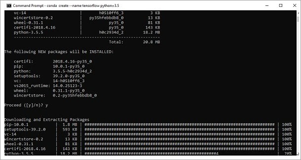
When it is effectively installed, examine the command prompt via the “conda” command. The implementation of the command is presented below:
Step #3: Apply the given command to commence the TensorFlow installation:


This downloads the required collections that are necessary for the setup of TensorFlow.
Step #4: When the environmental setup is successful, the activation of the TensorFlow module is crucial.


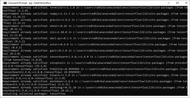
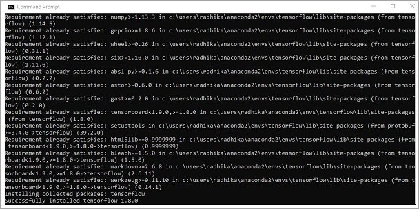
Step #5: Pip can be used to install “TensorFlow” in the system. The commands used are:

And


Once the installation is successful, it is a must to know the sample program implementation of TensorFlow.
Now that TensorFlow is properly installed and imported into your workspace, it’s time to focus on your data. Take time to explore and comprehend your data properly before modeling the neural networks.
Data Exploration
It’s time to download the dataset. Once the download is complete, the data needs to be imported into your workspace.
Let’s begin with the lines of code that emerge under the User-Defined Function (UDF) load_data():
- The foremost step is to settle your ROOT_PATH. This is where the directory is created with the training as well as the test data.
- Then certain paths can be added to the ROOT_PATH, with the assistance of the join() function. These two paths can be stored in the train data directory and test data directory.
- Afterward, the load_data() function can be named and forwarded to the train data directory to it.
- Now, the load_data() function begins by collecting the subdirectories that are available in the train data directory. It can do so with the assistance of list conception, which is a natural method for assembling lists. Essentially, it informs you that if something is found in the train data directory, you’ll need to include that in the list. Don’t forget that every subdirectory depicts a label.
- Then you are required to go through the subdirectories. Firstly, set two lists, labels, and images. Later, collect the various subdirectory paths along with the image file names that are reserved in the subdirectories. Then the data can be gathered in the two lists with the append() function.
def load_data(data_directory):
     directories = [d for d in os.listdir(data_directory)
                  if
os.path.isdir(os.path.join(data_directory, d))]
       labels = []
       images = []
       for d in directories:
            label_directory = os.path.join(data_directory, d)
            file_names = [os.path.join(label_directory, f)
                   for f in os.listdir(label_directory)
                   if f.endswith(".ppm")]
            for f in file_names:
                images.append(skimage.data.imread(f))
                labels.append(int(d))
       return images, labels
ROOT_PATH = "/your/root/path"
train_data_directory = os.path.join(ROOT_PATH, "TrafficSigns/Training")
test_data_directory = os.path.join(ROOT_PATH, "TrafficSigns/Testing")
images, labels = load_data(train_data_directory)
Visualizing the Data
When the data mainly involves images, visualizing it is an effective way to explore it.
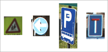
Let’s examine some traffic signs:
- The first thing that needs to be ensured is that the pyplot module of the matplotlib is imported under a common alias plt.
- Next, a list with four random numbers is to be made. These numbers will be utilized to choose traffic signs from the arrangement of the images that you have analyzed in the prior segment.
- After this will be done for every component in the extent of that list, from 0 to 4, subplots are going to be made, though without axes. In the subplots, a particular image will be presented from the arrangement of images that corresponds with the number at the index. In the end, the subplots will be adjusted so that there’s sufficient breadth between them.
- The final thing that is left is to show the plot using the show() function.
# Import the `pyplot` module of `matplotlib`
import matplotlib.pyplot as plt

# Determine the (random) indexes of the images that you want to see
traffic_signs = [300, 2250, 3650, 4000]

# Fill out the subplots with the random images that you defined
for i in range(len(traffic_signs)):
    plt.subplot(1, 4, i+1)
    plt.axis('off')
    plt.imshow(images[traffic_signs[i]])
    plt.subplots_adjust(wspace=0.5)
plt.show()

[image source]
As you might have guessed from the labels, the signs vary from each other. These images are different in size.
You can play around with the numbers that are held in the list of traffic_signs and proceed through this examination. This is a vital observation that you will be required to address when you are working towards influencing your data so that it can be fed to the neural networks.
You can confirm the hypothesis of the varying sizes by printing the shape, and the lowest and highest value of the certain images that are integrated into the subplots.
The following code highly mirrors the one that was used to form the above plot but is different as the sizes and images will be substituted and not just plotted together:
# Import `matplotlib`
import matplotlib.pyplot as plt

# Determine the (random) indexes of the images
traffic_signs = [300, 2250, 3650, 4000]

# Fill out the subplots with the random images and add shape, min and max values
for i in range(len(traffic_signs)):
    plt.subplot(1, 4, i+1)
    plt.axis('off')
    plt.imshow(images[traffic_signs[i]])
    plt.subplots_adjust(wspace=0.5)
    plt.show()
    print("shape: {0}, min: {1}, max:
{2}".format(images[traffic_signs[i]].shape,

images[traffic_signs[i]].min(),
images[traffic_signs[i]].max()))
Extracting Features
Now that the data is completely explored, it’s time to extract features. When you are aware of the things you need improvement in, you can manipulate the data so that it’s prepared to be fed to the neural networks or whatever model you want to feed it to.
We need to first begin with deriving some features, such as resizing the images, and the images that are held in the arrangement of the images will be transformed to grayscale.
The color transformation will be done as the color doesn’t have much value while classifying. Color only plays an important role during detection and in those instances, transformation is not necessary.
Resizing Images
To handle the varying sizes of the images, the images will need to be resized. This can be done easily with the help of the skimage or Scikit-Image library, which is a set of image processing algorithms.
In this, the transform module will be really helpful as it provides a resize() function. A list of comprehension will be required again for resizing each image to 28 by 28 pixels.
You’ll notice that the way to form the list, for every image found in the arrangement of the images, the modification operation that is taken from the skimmage library will be executed. Eventually, the results will be stored in the images28 variable.
# Import the `transform` module from `skimage`
from skimage import transform

# Rescale the images in the `images` array
images28 = [transform.resize(image, (28, 28)) for image in images]
Examine the result of the resizing operation by using the code again that was utilized earlier to plot the 4 random images using the traffic_signs variable. Remember to replace all references from images to images28.
Image Transformation to Grayscale
As mentioned earlier, the color of the images matters less when figuring out a classification question. Therefore, it’s also necessary to modify the images to grayscale. Similarly, with resizing, you can rely on the Scikit-Image library. In this, the color module with its rgb2gray() function will be used. This will be simple.
However, keep in mind to transform the images28 variable back to an arrangement, as the rgb2gray() function foresees an arrangement as an argument.
# Import `rgb2gray` from `skimage.color`
from skimage.color import rgb2gray

# Convert `images28` to an array
images28 = np.array(images28)

# Convert `images28` to grayscale
images28 = rgb2gray(images28)
Make sure to inspect the results of the grayscale transformation twice by plotting some of the images. The code can be used again and some of it can be adjusted to present the modified images:
import matplotlib.pyplot as plt

traffic_signs = [300, 2250, 3650, 4000]

for i in range(len(traffic_signs)):

    plt.subplot(1, 4, i+1)
    plt.axis('off')
    plt.imshow(images28[traffic_signs[i]], cmap="gray")
    plt.subplots_adjust(wspace=0.5)

# Show the plot
plt.show()
Other operations that could have been conducted on the data involve data augmentation (rotating, blurring, shifting, brightness changing). A complete pipeline of manipulating data operations could also be set up, through which the images can be sent.
Deep Learning with TensorFlow
Now that the data is explored and manipulated, you can build your neural network architecture using the TensorFlow package.
Also Read =>> Difference between Deep Learning and Machine Learning
Modeling the Neural Network
It’s time to construct your neural network, layer by layer. If not done previously, import TensorFlow into your workspace under the common alias tf. Now you can initialize the graph using Graph(). This function is used to describe the computation. The graph only describes the operation you are required to be working on later.
In this, a default context is to be set up using the as_default(), this returns a context manager that makes a particular graph the default graph. This method is used to generate various graphs using the same process. This function provides you with a global default graph in which all operations will be included if a new graph is not created precisely.
Now, you can add operations to the graph. Initially, the model is built up, then it is assembled, a loss function is defined, an optimizer, and a metric.
All of these steps occur at once while working with TensorFlow:
#1) Initially, the placeholders are defined for inputs and labels because the real data can’t be put in yet. Placeholders are values that are not allocated and will be set up by the session when worked on it. When the session is operated, these placeholders will receive the values of the dataset that is passed in the run() function.
#2) Then the network is built. The input is flattened using the flatten() function first. This provides an array of shapes.
#3) When the input is flattened, a completely linked layer creates logits of size. Logits is a function that works on the unscaled output of the prior layers, and that utilizes the comparative scale to comprehend that the units are linear.
#4) As the perceptron with the multiple layers is built out, the loss function can be defined. The option for the loss function entirely relies on the task. You will require:
sparse_softmax_cross_entropy_with_logits()
#5) The sparse softmax cross entropy between logits and labels, is calculated with this. To put it simply, the probability error is in separate categorization tasks, where the categories are mutually exclusive. This indicates that every entry is in a single category.
Here, a traffic sign can only contain an individual label. Whereas regression is used for predicting constant values, categorization is used to predict discrete values or categories of data points. This function is completed with reduce_mean(), which calculates the mean of elements over measurements of a tensor.
#6) A training optimizer is also defined. The most renowned optimization algorithms are Stochastic Gradient Descent (SGD), ADAM, and RMSprop.
Particular parameters need to be adjusted, like the learning rate or momentum, which depends on the chosen algorithm. In this case, the ADAM optimizer is picked, for which the learning rate is defined at 0.001.
#7) In conclusion, the execution of operations is going to be set, before going over to the training.
# Import `tensorflow`
import tensorflow as tf

# Initialize placeholders
x = tf.placeholder(dtype = tf.float32, shape = [None, 28, 28])
y = tf.placeholder(dtype = tf.int32, shape = [None])

# Flatten the input data
images_flat = tf.contrib.layers.flatten(x)

# Fully connected layer
logits = tf.contrib.layers.fully_connected(images_flat, 62, tf.nn.relu)

# Define a loss function
loss = tf.reduce_mean(tf.nn.sparse_softmax_cross_entropy_with_logits(labels = y,

logits = logits))

# Define an optimizer
train_op = tf.train.AdamOptimizer(learning_rate=0.001).minimize(loss)

# Convert logits to label indexes
correct_pred = tf.argmax(logits, 1)

# Define an accuracy metric
accuracy = tf.reduce_mean(tf.cast(correct_pred, tf.float32))
Your first neural network with TensorFlow is successfully formed. The values of most of the variables can also be printed, if you want to get a rapid summary of your code:
print("images_flat: ", images_flat)
print("logits: ", logits)
print("loss: ", loss)
print("predicted_labels: ", correct_pred)
Conclusion
In this TensorFlow Tutorial, we thoroughly covered what TensorFlow is. TensorFlow is a software library for machine learning applications. It was designed to enable developers to build custom applications that can learn and optimize their own performance using artificial neural networks and deep learning techniques.
Then we went over its APIs and found out that it has two types of APIs; low-level APIs and high-level APIs. To better understand TensorFlow, we explained its applications. We clarified how to properly install TensorFlow in your system.
At the end of this TensorFlow Tutorial, we unfolded how deep learning works with TensorFlow.


