


Quickly understand all about Decision Tree in Machine Learning with examples. Discover the various terminologies, pros, cons, learning algorithms & applications in Decision trees from here:
Based on information in the digital data set, decisions or predictions made by a computer algorithm are called a decision tree flowchart. By using the word supervised learning, we can understand the algorithm used for deciding based on past outcomes.
Every leaf node represents a class label and branches depict a conjunction of features. The path is known as classification rules from root to leaf. The decision tree can be built by leveraging CART (Classification and Regression Tree algorithm).
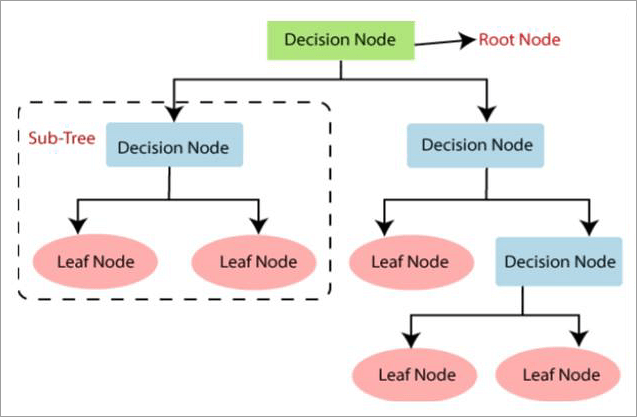
The decision tree is a graphical representation for getting all the solutions to a problem under a defined set of circumstances. The internal nodes depict the dataset’s features, branches define the decision rules and the leaf node represents the outcome.
Table of Contents:
An Introduction to Decision Tree Algorithm in ML

The leaf node does not contain any branches, while decision nodes have multiple branches and they make any decision. A decision tree asks a simple question and based on it, further splitting of the tree into sub-trees is done.
Decision tree is used in data mining, machine learning, and statistics. They are non-parametric supervised learning methods that can be used for both regression and classification tasks. The algorithmic approach constructs the decision tree based on distinct conditions and finds a way of splitting the data.
In this article, we are going to explore the terminologies, advantages, disadvantages, learning algorithms, and applications of decision trees while leveraging machine learning technology.
[image source]
Terminologies Used in a Decision Tree
- Root Node: From the root node, the entire dataset is represented. It is the point from where the decision tree starts and gets divided into homogenous sets.
- Splitting: Based on the decision criterion, dividing the node into sub-nodes. For creating subsets of data, selecting a feature is important.
- Leaf Nodes: These final output nodes cannot be further segregated.
- Parent Node: The root node of a decision tree is known as the parent node and sub-nodes are classified as the child node.
- Child Node: Nodes that are created by splitting from the parent node.
- Branches: While deciding, links between the nodes are called branches.
- Pruning: The process of removing nodes or branches from a decision tree is called pruning. By doing it, generalization can be improvised and overfitting can be removed. Reduced error and cost complexity are the two types of pruning technology that are used vastly.
- Decision Criterion: It is a type of rule that determines how the data should be split. Against a given threshold, it compares feature values.
Steps for Making a Decision Tree
- Starting from the root node of a tree, the algorithm is used for predicting the class of a dataset.
- First, the root node is created that contains the entire dataset. For that, a list of rows needed for consideration needs to be fetched.
- Second, using an attribute selection measure, the best attribute from the dataset can be selected. Adjacently, the uncertainty of the dataset or Gini impurity needs to be calculated.
- Third, the root node can be divided into subsets known as sub-nodes. All of these subsets contain possible values. Partition of rows can be done based on true and false rows.
- Based on the partition of data and Gini impurity, information gain can be calculated.
- Updation of information gain is required based on each question asked.
- Fourth, continuously new decision trees should be created. Continue the segregation until a stage is reached where nodes can’t be further divided. The finalized nodes are called leaf nodes.
We can understand it much better with the help of an example:
There is a candidate. There are two situations for him. Either he can accept the offer or reject the offer. In this scenario, salary is the root node of a decision tree. The root node gets split into the next decision tree node.
One node represents the distance of the office from home and another leaf represents the corresponding classification label. Further moving on, the decision tree node gets split into decision nodes i.e. Cab facility and leaf node (defining the class label). After that, the decision tree node gets split further into child node (accepted and declined the offer)
Example of Decision Tree:

Why a Decision Tree
While creating a machine learning model, choosing the perfect algorithm according to the dataset is one of the most important things. From the various algorithms used in machine learning, decision trees usually are preferred because of mimic human thinking ability. By leveraging the decision tree structure, one can easily grasp the logic behind each node.
How decision tree is formed?
Based on different values of distinct attributes, continuous data is partitioned while forming a decision tree. The decision of which attribute algorithm to use for splitting the data at each internal node is determined by either Gini impurity or information gain.
This process of splitting the data continues until the maximum depth is reached or by having a minimum number of instances in a leaf node.
Decision Tree Approach
The decision trees use a tree-like structure for solving the problems. The leaf node is represented as a class label, while the attribute depicts the internal node of a tree. The decision tree represents the boolean function on discrete attributes.
Here, we are going to discuss assumptions made during the creation of the decision tree:
- The records are distributed continuously based on attribute values.
- For ordering the attributes as roots, statistical methods are used while creating the decision tree.
- Before building the model, the feature values are used. The feature values are categorical and they need to be discretized if they’re continuous.
Attribute Selection
While implementing a decision tree, the best attribute for the root node and sub-node needs to be selected. It is one of the major challenges in decision trees. Leveraging Attribute Selection Measure (ASM), we can easily select the best attribute that fits the node or sub-node.
There are two popular attribute selection measures:
Gini Impurity
- Pure: It means that the entire data belongs to a particular class.
- Impure: Impure means the data belongs to distinct classes.
There are two most popular attribute selection measures:
Gini Index
It is a measure of impurity or inequality of a distribution. It varies from 0 to 1. While 0 represents perfect equality and 1 depicts perfect inequality. A low Gini index represents pure distribution while a high Gini index depicts impure distribution.
The Gini index is more sensitive to changes in class probabilities and is faster to compute. The Gini index can be calculated by using the formula as shown below:
Gini Index = 1 –∑jPj^(2)
Information Gain
The entropy changes when the partition of training instances into smaller subsets is done. A measure of change in entropy is known as information gain. Information gain allows the derivation of information about a particular feature of a class.
The splitting of nodes and building of decision trees are considered under the value of information gain. The nodes containing the highest information are spilted first.
Information Gain = Entropy (s) – Weighted Avg * Entropy of each feature
Entropy is a measure of measuring the impurity in an attribute. Using the formula given below, entropy can be calculated:
Entropy (s) = P (yes) log 2 P (yes) – P (no) log 2 P (no)
Here, S is the number of samples
P (no): Probability of no
P (yes): Probability of yes
Let’s have a look at one of the decision tree algorithms to better understand the root node, leaf node, attribute, subsets, and recursive splitting.
- Root Node: It consists of the entire dataset.
- Leaf Node: It includes the types of activities, i.e. working, sleeping, eating, etc.
- Attribute: It defines the outlook.
- Subsets: This includes the splitting of attributes. For example, sunny, rainy, and so on.
- Recursive Splitting: The dividing of a subset is called recursive splitting. The Sunny can be further classified according to humidity.
Types of Decision Trees
There are two main types of decision tree:
#1) Classification: The trees predicting categorical variables such as A, B, C, D, and E are called classification trees.
Decision Tree Classifier
On a given dataset, performing multi-class classification is called a decision tree classifier. The input is taken into two arrays. Array X is holding training samples while array y is holding integer values. It is capable of both binary and multiclass classification.
From sklearn import tree
X = [[1,1], [2,2]]
Y = [1,2]
Clf = tree.decisiontreeclassifier ()
Clf =clf.fit (X, Y)
After it, the model can be used for predicting the class of samples.
Clf.predict ([[2.,2.]])
Array ([1])
#2) Regression: The trees predicting numeric outcomes are known as regression trees. Leveraging the DecisionTreeRegression Class, the regression problems of a decision tree can be solved. As per the classification setting, two arrays will be taken. But, in this case, array y will take floating point values instead of an integer.
From sklearn import tree
X = [ [2,2], [4,4]]
Y = [3.0, 4.5]
Clf = tree.decisiontreeregressor ()
Clf = clf.fit (x,y)
clf.predict([3,3])
Array ([3.0])
Data Format: The data comes in the format as shown below:
(x, Y) = (x1, x2, x3, x4, x5, x6, ……xK, Y)
The vector X denotes features, while Y defines the target variable for generalizing, classifying, and understanding.
How to build a decision tree?
Based on training data, the decision tree in machine learning can be built:
Training _data = [
['Apple', '1', 'Red']
['Grape', '2', 'Green']
['Banana', '3', 'Yellow']
['Strawberry', '4', 'White']
Header = ["Label", "Diameter", "Color"]
The first column is labeled.
The last two columns are features.
Tree = Build_tree (training data)
Print (Tree)
Here is the output delivered based on the input:
Is diameter >= 3?
—-----> true :
Is color = = Yellow?
 —----> true :
Predict { 'Banana' : 3 }
This process continues until and unless a leaf node is reached where information gain is zero and further splitting of nodes is not possible. The entire training data is divided into true and false rows, as shown above in the output.
Python Implementation of Decision Tree
With the classification models like logistic regression and KNN SVM, we can build the decision tree using Python. For this, we can use the “training_data.csv” type of data.
Below are the steps mentioned for implementing Python while creating the decision tree.
#1) Data Pre-Processing: Here is the code that can be used for data pre-processing.
import libraries
import numpy as nmn
import matplotlib.pyplot as matpy
import pandas as pan
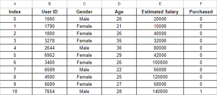
importing datasets
data_set= pd.read_csv('training_data.csv')
Extracting dependent and independent variable
x= data_set.iloc[:, [3,4]].values
y= data_set.iloc[: 5].values
Dataset splitting for training and testing
from sklearn.model_selection
import test_train_split
x_train, x_test, y_train, y_test= train_test_split(x, y, test_size= 0.5, random_state=1)
Scaling of features
from sklearn.preprocessing
import StandardScaler
st_x= StandardScaler()
x_test= st_x.fit_transform(x_test)
y_test= st_x.transform(x_train)
Preprocessing Data:
#2) Fitting a Decision Tree Algorithm
From the sklearn.tree library, the decision tree classifier can be imported. With the help of the training data set, we can fit the model:
Getting the training set fit into decisiontreeclassifier
from the sklearn.tree
import DecisionTreeClassifier
classifier= DecisionTreeClassifier (criteria ='entropy', random_state=1)
classifier.fit (x_train, y_train)
Output:
DecisionTreeClassifier
(class_weight= 0, criteria= 'entropy', max_depth = 0,
Max_features = 0, max_leaf_nodes = 0,
Min_impurity_decrease = 0.0, min_impurity_split = 0,
Min_samples_leaf = 2, min_samples_split = 4,
Min_weight_fraction_leaf = 0.1, presort = False,
Random_state = 0, splitter = 'best')
In the above code, we have used two parameters for classifying the object:
- Random_state = 0: For generating the random states, we have used the random_state parameter.
- Criteria = entropy: For measuring the quality of spilled, criteria are used. It is calculated through information gain in an entropy.
Predicting the Results: In the below code, we have created a new prediction vector z_pred. Through it, we can predict the results of the test data set.
Predicting the result of a test set
z_pred= classifier.predict(y_test)
Predicted output and real test output:
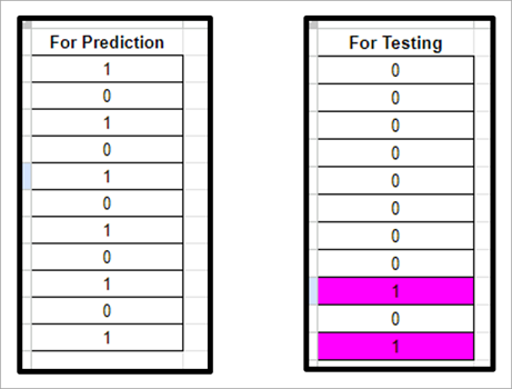
In the above image, we can see that there are values that differ from real vector values.
#3) Test Accuracy of Results:
Using a confusion matrix, the number of correct as well as incorrect predictions can be known.
Below is the code for testing the accuracy:
Confusion Matrix
from sklearn.metrics
import confusion_matrix
con= confusion_matrix (x_test, z_predict)
Predicted output and real test output:
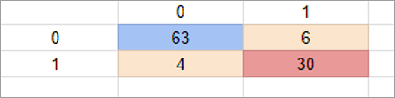
In the above image, we can see the number of correct and incorrect predictions. Therefore, we can conclude that the decision tree classifier makes a good prediction as compared to other classifier models.
#4) Visualizing the Results: Using the logistic regression model, we can visualize the training data set results. Below is the code that can be used for visualizing the training data set.
For visualizing the results of the training test set
For visualizing the results of the training test set
from matplotlib.colors
import ListedColormap
y_set, y_set = y_train, y_train
y1, y2 = nm.meshgrid (nm.arrange(start = y_set[:, 0].min() - 1, stop = y_set[:, 0].max() + 1, step = 0.02)
nm.arrange(start = y_set[:, 1].min() - 1, stop = y_set[:, 1].max() + 1, step = 0.02))
mtp.contourf(y1, y2, classifier.predict(nm.array([y1.ravel(), y2.ravel()]).T).reshape(y1.shape),
alpha = 0.80, cmap = ListedColormap (('red','yellow' )))
mtp.ylim(y1.min(), y1.max())
mtp.ylim(y2.min(), y2.max())
for, j in enumerate(nm.unique(y_set)):
mtp.scatter(x_set[y_set == j, 0], y_set[y_set == j, 1]
c = ListedColormap (('red', 'yellow'))(i), label = j)
mtp.title ('Decision Tree Algorithm (Training set)')
mtp.ylabel ('Age')
mtp.ylabel ('Estimated Salary')
mtp.legend()
mtp.show()
Advantages & Disadvantages
Here are the advantages of the Decision Tree:
- It is easy to handle and understand through visualization.
- Able to handle both numerical and categorical data
- Highly mismanaged data can also be used. It does not require any cleaning or standardization of data.
- For training, it does not require too much amount of time.
- Multi-output problems can be easily handled with the decision tree.
- Little preparation of the dataset is required as dummy variables can be created, blank values can be removed and data normalization can be done.
- Using statistical tests, the model can be validated. By testing, the reliability of a model can be predicted.
- The number of data points used for training the tree can calculate the cost of a tree.
Disadvantages of Decision Tree:
- During parameter tuning, needs to be more precise.
- Overfitting of the model is expected if the dataset is not balanced and some classes dominate.
- The decision tree in machine learning has several layers that make it complex to understand. They are neither continuous nor smooth. Therefore, they’re not for extrapolation.
- Small variations in data can lead to instability in the decision tree. Often, it may result in the generation of a completely new tree. This problem can be mitigated with the usage of an ensemble in decision trees.
- While dealing with unbalanced data, potential bias can happen.
- For problems like XOR, multiplexer, or parity, these concepts are hard to understand by the decision tree.
How to avoid overfitting in the decision tree model
Overfitting can be avoided by stopping the tree-building process at an early stage. It is also known as pre-pruning decision trees. At every stage of splitting, a cross-validation error is measured. If it is not significantly decreasing, then the splitting needs to be stopped.
Major two pruning techniques that can be used are discussed below:
- Minimum Tree: The decision tree is pruned where the cross-validated error is minimum.
- Smallest Tree: At the minimum error point, the tree is pruned back slightly. With the help of cross-validation error, one can create a decision tree with one standard error of the minimum error.
By avoiding overfitting, the complexity of a tree can be reduced. It overall improves the accuracy of the decision tree model.
Frequently Asked Questions
1. What is a decision tree in machine learning?
Based on input features, a decision tree in machine learning is a supervised learning algorithm. It makes decisions based on attributes. It is in the form of a tree-like structure where the nodes represent the decision taken by the model.
2. What are the hyperparameters in the decision tree?
Here, are a few of the hyperparameters used in the decision tree:
Min Samples Leaf: Minimum samples that are required in a leaf node.
Criterion: For measuring the quality of the split, the criterion function is used.
Min Samples Split: The minimum number of samples required to split an internal node
Max Depth: The maximum depth of a decision tree
3. What is entropy in a decision tree?
Entropy means the disorder or impurity within a dataset. It assists in guiding the algorithm for making informative splits. It also quantifies the uncertainty associated with classifying the instances.
4. What are the major issues in decision tree learning?
Limited generalization, small data changes, and overfitting are some of the major issues in decision tree learning. For creating robust decision tree models, proper tuning, pruning, and handling imbalanced data can mitigate these challenges.
5. Can a decision tree be used for predicting?
Using the previous data, the classification model was optimized for obtaining accuracy. Once we test and optimize the decision tree, we can further use it for predicting future outcomes.
6. How can we use a decision tree in machine learning?
It is an effective way of finding all the solutions related to a problem. It assists the developers in finding all the consequences of a decision. While an algorithm can access the data, a decision tree leveraging machine learning technology can easily predict future outcomes.
Conclusion
Based on input data, the decision tree can be created as a tree-like structure. Leveraging decision tree understanding can be very easy. Before deep diving and understanding the applications of decision trees, it is important to understand the terminologies and processes for using them in distinct scenarios.
Decision trees are valuable for both regression and categorization tasks, as they provide versatility, interpretability, and ease of simple visualization. Overfitting, limited generalization, and sensitivity to small data changes are some challenges in creating a decision tree.
Further Reading => Decision Tree Algorithm In Data Mining
Was this helpful?
Recommended Reading
-

To help you get ready for your interview, this tutorial contains popular Machine Learning questions and answers, complete with explanations. In this tutorial, we have discussed the most asked machine learning interview questions and answers. The interview questions listed below are very useful for preparation for jobs as a machine…
-

List and Comparison of the best paid as well as open source free Machine Learning Tools: What is Machine Learning? With the help of machine learning systems, we can examine data, learn from that data, and make decisions. Machine learning involves algorithms and a Machine learning library is a bundle…
-
What is the Difference Between Data Mining Vs Machine Learning Vs Artificial Intelligence Vs Deep Learning Vs Data Science: Both Data Mining and Machine learning are areas which have been inspired by each other, though they have many things in common, yet they have different ends. Data mining is performed…
-
Here is a comprehensive guide that will help you understand the difference between Deep Learning and Machine Learning, and gain practical hands-on experience: In the previous tutorial, we learned how to perform Data Visualization, K-means Cluster Analysis, and Association Rule Mining using WEKA Explorer Look at different career opportunities in…
-
This Genetic Algorithm Tutorial Explains what are Genetic Algorithms and their role in Machine Learning in detail: In the Previous tutorial, we learned about Artificial Neural Network Models – Multilayer Perceptron, Backpropagation, Radial Bias & Kohonen Self Organising Maps including their architecture. We will focus on Genetic Algorithms that came…
-
This Tutorial Explains What is Machine Learning, How Does It Work, Applications of ML and The Comparison of Machine Learning Vs Artificial Intelligence: Machine Learning is a field in computer science that learns from experience without being programmed. It is a part of Artificial Intelligence, or we can say that…
-
Read This In-depth Review of the Top Machine Learning Companies Across The World to Select the Best ML Company Based on Pricing, Features & Comparison: Machine Learning (ML) is the concept that helps machines to learn from data. It is done by finding the pattern in data. Thus the performance…
-
This Tutorial Explains The Types of Machine Learning i.e. Supervised, Unsupervised, Reinforcement & Semi-Supervised Learning With Simple Examples. You Will Also Learn the Differences Between Supervised Vs Unsupervised Learning: In the Previous Tutorial, we learned about Machine Learning, its working, and its applications. We have also seen a comparison of…


